IPYVOLME: 3D Plotting for Python in the Jupyter Notebook based on IPython Widgets using WebGL

Introduction

Ipyvolume is a Python library designed for visualizing 3D data directly in Jupyter notebooks with minimal configuration and effort. Built on IPython widgets and WebGL, it allows users to create interactive 3D visualizations, such as scatter plots, surface plots, volume rendering, and more. Ipyvolume leverages the power of three.js, a JavaScript library for rendering OpenGL/WebGL-based graphics, ensuring fast and interactive 3D rendering in the browser.

The primary use of Ipyvolume is for visualizing 3D volumes and glyphs (like 3D scatter plots) within Jupyter notebooks. It’s especially useful in scientific computing, data science, and other domains that require in-depth visual exploration of complex 3D datasets. For example, it provides volume rendering of 3D arrays, similar to how matplotlib’s imshow renders 2D arrays, allowing users to visualize volumetric data interactively.

One of the key features of Ipyvolume is its ease of use. Users can quickly create interactive visualizations from numpy arrays or 3D datasets with just a few lines of code. Moreover, Ipyvolume’s volshow function is tailored for 3D arrays, while other plotting libraries like yt, VTK, and Mayavi can handle more complex, mature, but potentially more difficult-to-use tasks.

Ipyvolume also supports other 3D visualizations such as scatter plots, quiver plots, mesh plots, and more. It’s especially useful for creating visualizations that allow users to interact with the data, rotating, zooming, and panning to explore the structure of the data from various angles.

In this blog we have made a real life model of the solar system using it as we will see ahead.

Installation

Using Pip

Conda/Anaconda

For Jupyter lab users

The Jupyter lab extension is not enabled by default (yet).

Pre-notebook 5.3

If you are still using an old notebook version, ipyvolume and its dependend extension (widgetsnbextension) need to be enabled manually. If unsure, check which extensions are enabled:

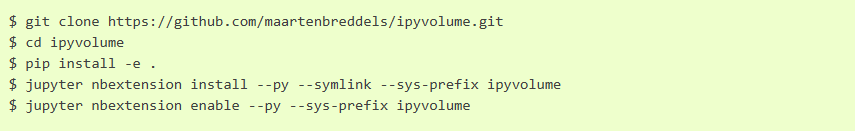
Developer installation

Key Features of ipyvolume

1. Seamless Integration with ipywidgets

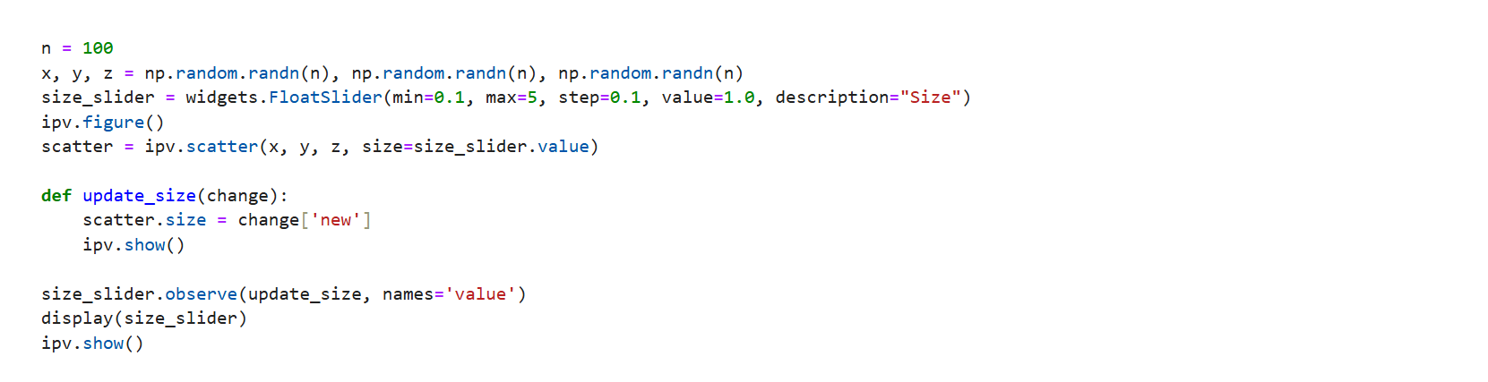
ipyvolume integrates effortlessly with ipywidgets, allowing users to enhance their 3D visualizations with interactive controls such as sliders, dropdowns, and buttons.

In the example below, we use an ipywidgets slider to dynamically adjust the size of points in a scatter plot created with ipyvolume:

import ipyvolume as ipv
import numpy as np
import ipywidgets as widgets
import matplotlib.pyplot as plt
import bqplot.scales
import pythreejs
from IPython.display import Image, display

2. Animating Time Series Data

ipyvolume enables dynamic 3D visualizations by supporting animations, making it ideal for representing time-varying data.

It allows users to animate objects over multiple frames and interactively explore how data evolves over time.

In the example below, we create an animated 3D quiver plot where vector directions change over time.

The animation_control function provides interactive playback options directly within Jupyter Notebook:

import ipyvolume as ipv
import numpy as np

n = 100
x, y, z = np.random.randn(n), np.random.randn(n), np.random.randn(n)
t = np.linspace(0, 2 * np.pi, 20)  # 20 time steps
u = np.sin(t)[:, None] * np.random.randn(n)
v = np.cos(t)[:, None] * np.random.randn(n)
w = np.sin(t * 2)[:, None] * np.random.randn(n)

ipv.figure()
quiver = ipv.quiver(x, y, z, u, v, w, size=5)

ipv.animation_control(quiver)
ipv.show()

3. Integration of bqplot, vaex, and ipyvolume for Interactive Data Visualizations

Combining the strengths of multiple libraries can yield powerful insights when working with large datasets. In this example, we demonstrate how to integrate vaex, bqplot, and ipyvolume in a Jupyter Notebook to explore NYC taxi data:

• vaex is utilized for fast and memory-efficient processing of large datasets, enabling quick data filtering, aggregation, and analysis.

• bqplot provides interactive, linked charting that can be used to complement the 3D visualizations.

• ipyvolume renders the processed data in a dynamic 3D space, where users can explore the spatial distribution of taxi trips.

In the example below, we use an ipywidgets slider to dynamically adjust the size of points in a plot. This interactivity allows you to explore different aspects of the data by changing visual parameters on the fly. We can further use ipyvolume to visualize it in 3D. But sometimes espesially for very large datasets 2D is better to vizualize.

4. 3D Line Plots for Trajectories and Curves

ipyvolume allows users to create smooth and interactive 3D line plots, which are useful for visualizing trajectories, paths, and mathematical curves.

By specifying the x, y, and z coordinates, we can plot curves in three-dimensional space with customizable colors and styles.

In the example below, we generate a 3D helix and visualize it using ipyvolume.plot():

import ipyvolume as ipv
import numpy as np

t = np.linspace(0, 4 * np.pi, 100)  # 100 points
x, y, z = np.sin(t), np.cos(t), t  # Helix curve

ipv.figure()
ipv.plot(x, y, z, color="red", linewidth=20)
ipv.show()

Examples using ipyvolume

These are some examples of different plots made using this library and have been taken from the documentation

First let us import all the neccessary libraries

import ipyvolume as ipv
import numpy as np
import ipywidgets as widgets
import matplotlib.pyplot as plt
import bqplot.scales
import pythreejs
from IPython.display import Image, display

A simple scatter plot

This code generates 1,000 random points in 3D space using a normal distribution and visualizes them using ipyvolume

N = 1000
x, y, z = np.random.normal(0, 1, (3, N))
fig = ipv.figure()
scatter = ipv.scatter(x, y, z)
ipv.show()

Plotting Surface

This code creates a 3D surface plot of a function f(u, v) -> (u, v, uv^2) using ipyvolume

# f(u, v) -> (u, v, u*v**2)
a = np.arange(-5, 5)
U, V = np.meshgrid(a, a)
X = U
Y = V
Z = X*Y**2

ipv.figure()
ipv.plot_surface(X, Z, Y, color="orange")
ipv.plot_wireframe(X, Z, Y, color="red")
ipv.show()

Texture mapping

This code applies a PNG image as a texture to a 3D mesh surface using ipyvolume. It downloads an image, maps it to the surface using UV coordinates, and animates the texture shift across 8 frames to create a dynamic effect. The scene is displayed in dark mode with no wireframe.

import PIL.Image
import requests
import io

url = 'https://vaex.io/img/logos/spiral-small.png'
r = requests.get(url, stream=True)
f = io.BytesIO(r.content)
image = PIL.Image.open(f)

fig = ipv.figure()
ipv.style.use('dark')
# we create a sequence of 8 u v coordinates so that the texture moves across the surface.
u = np.array([X/5 +np.sin(k/8*np.pi)*4. for k in range(8)])
v = np.array([-Y/5*(1-k/7.) + Z*(k/7.) for k in range(8)])
mesh = ipv.plot_mesh(X, Z, Y, u=u, v=v, texture=image, wireframe=False)
ipv.animation_control(mesh, interval=800, sequence_length=8)
ipv.show()

Basic animation

This code creates an animated 3D scatter plot using ipyvolume, where spheres oscillate based on a decaying cosine wave. The grid points (x, y) determine radial distances r, and the height z evolves over 15 time steps to create a wave-like animation.

# create 2d grids: x, y, and r
u = np.linspace(-10, 10, 25)
x, y = np.meshgrid(u, u)
r = np.sqrt(x**2+y**2)
print("x,y and z are of shape", x.shape)

# and turn them into 1d
x = x.flatten()
y = y.flatten()
r = r.flatten()

# create a sequence of 15 time elements
time = np.linspace(0, np.pi*2, 15)
z = np.array([(np.cos(r + t) * np.exp(-r/5)) for t in time])
print("z is of shape", z.shape)

# draw the scatter plot, and add controls with animate_glyphs
ipv.figure()
s = ipv.scatter(x, z, y, marker="sphere")
ipv.animation_control(s, interval=200)
ipv.ylim(-3,3)
ipv.show()

x,y and z are of shape (25, 25)
z is of shape (15, 625)

Animated quiver

This code visualizes an animated 3D vector field using ipyvolume. It loads a predefined animated stream dataset, where each particle has position (x, y, z) and velocity (vx, vy, vz) over time. The quiver plot (ipv.quiver) animates 200 particles over 50 time steps, displaying red arrows that represent their motion in 3D space.

import ipyvolume.datasets
stream = ipyvolume.datasets.animated_stream.fetch()
print("shape of steam data", stream.data.shape) # first dimension contains x, y, z, vx, vy, vz, then time, then particle

fig = ipv.figure()
# instead of doing x=stream.data[0], y=stream.data[1], ... vz=stream.data[5], use *stream.data
# limit to 50 timesteps to avoid having a huge notebook
q = ipv.quiver(*stream.data[:,0:50,:200], color="red", size=7)
ipv.style.use("dark") # looks better
ipv.animation_control(q, interval=200)
ipv.show()

shape of steam data (6, 200, 1250)

Using scales

This code creates a 3D scatter plot with logarithmic scaling on the x-axis using ipyvolume and bqplot.scales

import bqplot.scales
N = 500
x, y, z = np.random.normal(0, 1, (3, N))
x = 10**x
r = np.sqrt(np.log10(x)**2 + y**2 + z**2)
scales = {
    'x': bqplot.scales.LogScale(min=10**-3, max=10**3),
    'y': bqplot.scales.LinearScale(min=-3, max=3),
    'z': bqplot.scales.LinearScale(min=-3, max=3),
}
color_scale = bqplot.scales.ColorScale(min=0, max=3, colors=["#f00", "#0f0", "#00f"])
fig = ipv.figure(scales=scales)
scatter = ipv.scatter(x, y, z, color=r, color_scale=color_scale)
ipv.view(150, 30, distance=2.5)
ipv.show()

Bar Charts

This code creates an animated 3D scatter plot in ipyvolume, where color and box size dynamically change based on a cosine-based wave function. The scatter points are box-shaped, with their height (y-dimension) varying over time, and color mapped to the oscillating values.

u_scale = 10
Nx, Ny = 30, 15
u = np.linspace(-u_scale, u_scale, Nx)
v = np.linspace(-u_scale, u_scale, Ny)
x, y = np.meshgrid(u, v, indexing='ij')
r = np.sqrt(x**2+y**2)
x = x.flatten()
y = y.flatten()
r = r.flatten()

time = np.linspace(0, np.pi*2, 15)
z = np.array([(np.cos(r + t) * np.exp(-r/5)) for t in time])
zz = z

fig = ipv.figure()
s = ipv.scatter(x, 0, y, aux=zz, marker="sphere")
dx = u[1] - u[0]
dy = v[1] - v[0]
# make the x and z lim half a 'box' larger
ipv.xlim(-u_scale-dx/2, u_scale+dx/2)
ipv.zlim(-u_scale-dx/2, u_scale+dx/2)
ipv.ylim(-1.2, 1.2)
ipv.show()

# make the size 1, in domain coordinates (so 1 unit as read of by the x-axis etc)
s.geo = 'box'
s.size = 1
s.size_x_scale = fig.scales['x']
s.size_y_scale = fig.scales['y']
s.size_z_scale = fig.scales['z']
s.shader_snippets = {'size':
 'size_vector.y = SCALE_SIZE_Y(aux_current); '
}

s.shader_snippets = {'size':
 'size_vector.y = SCALE_SIZE_Y(aux_current) - SCALE_SIZE_Y(0.0) ; '
}

s.geo_matrix = [dx, 0, 0, 0,   0, 1, 0, 0,   0, 0, dy, 0,  0.0, 0.5, 0, 1]

# since we see the boxes with negative sizes inside out, we made the material double sided
s.material.side = "DoubleSide"
# Now also include, color, which containts rgb values
color = np.array([[np.cos(r + t), 1-np.abs(z[i]), 0.1+z[i]*0] for i, t in enumerate(time)])
color = np.transpose(color, (0, 2, 1)) # flip the last axes
s.color = color
ipv.animation_control(s, interval=200)

Animation with shadow

This code visualizes an animated 3D vector field using ipyvolume, where quiver arrows represent particle motion from a dataset. It adds lighting effects and planes for better visualization while using a dark theme for contrast. The animation updates at 200ms intervals to show the evolution of the vector field over time.

import ipyvolume.datasets
stream = ipyvolume.datasets.animated_stream.fetch()
print("shape of steam data", stream.data.shape) # first dimension contains x, y, z, vx, vy, vz, then time, then particle

fig = ipv.figure()
# instead of doing x=stream.data[0], y=stream.data[1], ... vz=stream.data[5], use *stream.data
# limit to 50 timesteps to avoid having a huge notebook
ipv.material_physical()
# q = ipv.quiver(*stream.data[:,0:200:10,:2000:10], color="red", size=7)
q = ipv.quiver(*stream.data, color="red", size=7)
ipv.style.use("dark") # looks better
m = ipv.plot_plane('bottom')
m = ipv.plot_plane('back')
m = ipv.plot_plane('left')
ipv
l = ipv.light_directional(position=[20, 50, 20], shadow_camera_orthographic_size=1, far=140, near=0.1);
ipv.animation_control(q, interval=200)
ipv.show()

shape of steam data (6, 200, 1250)

Interactive Solar System made by us

In this section, we demonstrate the power of ipyvolume with a fully interactive 3D visualization of our Solar System. Using real astronomical data, we’ve modeled the eight planets; complete with their colors, sizes, densities, and orbital characteristics to create a realistic simulation of their motion around the Sun.

What Does This Example Showcase?

• Real-World Data Integration:

  All planetary parameters (such as diameters, orbital distances, and inclinations of orbits) are based on actual measurements, scaled appropriately to create a visually engaging model.The data is taken from all trusted sources, linked in references.
• 3D Rendering with ipyvolume:

  Planets are rendered as 3D spheres using scatter plots, while their orbits are depicted as smooth ellipses drawn with line plots. This combination brings a tangible sense of depth and realism to the simulation.
• Interactive Controls with ipywidgets:

  A dropdown menu lets you select any planet to view its detailed information (coordinates, size, density, and orbital period) at a given time frame. An accompanying slider lets you navigate through time, watching the dynamic motion of each planet along its orbit.
• Dynamic Animation:

  The animation control continuously updates the visualization, simulating the planets’ movements as they orbit the Sun, demonstrating ipyvolume’s capability for smooth, interactive, time-series animations.

Run the cell below to see the interactive Solar System in action and explore how ipyvolume can transform your data visualizations!

# Planet names
planets = ["Mercury", "Venus", "Earth", "Mars", "Jupiter", "Saturn", "Uranus", "Neptune"]
colors_rgb = np.array([
    (0.55, 0.55, 0.55),  # Mercury - Grayish
    (0.98, 0.82, 0.15),  # Venus - Pale yellow
    (0.0, 0.4, 1.0),     # Earth - Deep blue with land reflections
    (0.8, 0.3, 0.1),     # Mars - Reddish brown
    (0.9, 0.6, 0.3),     # Jupiter - Orange with brown bands
    (0.9, 0.8, 0.6),     # Saturn - Pale yellowish-beige
    (0.4, 0.8, 0.9),     # Uranus - Cyan/Light Blue
    (0.1, 0.1, 0.7)      # Neptune - Deep Blue
])
densities = np.array([5.43, 5.24, 5.51, 3.93, 1.33, 0.69, 1.27, 1.64])
alpha_values = 0.3 + 0.7 * (densities / np.max(densities))

semi_major_axes = np.array([58, 108, 149, 228, 778, 1427, 2871, 4497])*(10**6)
eccentricities = np.array([0.206, 0.007, 0.017, 0.093, 0.048, 0.056, 0.046, 0.010])
inclinations = np.array([7.00, 3.4, 0.00, 1.8, 1.3, 2.5, 0.8, 1.8]) * (np.pi / 180)  # Convert to radians

real_distances = np.array([0.31, 0.72, 0.98, 1.38, 4.95, 9.01, 18.28, 29.80])*1.496*(10**8)
real_diameter = np.array([4878, 12100, 12756, 6794, 142800, 120000, 52400, 48400])
real_radii = real_diameter/2
sun_radius = 696340

scale_factor_distance = 0.00001
scale_factor_size = 0.0001

scaled_distances = scale_factor_distance*real_distances
scaled_radii = scale_factor_size*real_radii

scaled_semi_major_axes = semi_major_axes * scale_factor_distance  # Scaled distances

orbital_periods = np.array([88, 225, 365, 687, 4333, 10759, 30687, 60190])

angular_speeds = 50*((2 * np.pi) / orbital_periods)
time = np.linspace(0, 1000 * np.pi, 6000)

x, y, z = [], [], []  # For x, y, z positions over time using elliptical orbits
for i in range(len(planets)):
    theta = angular_speeds[i] * time  # Angle for each time step
    r = (scaled_semi_major_axes[i] * (1 - eccentricities[i]**2)) / (1 + eccentricities[i] * np.cos(theta))

    x_orbit = r * np.cos(theta)
    y_orbit = r * np.sin(theta)
    z_orbit = np.zeros_like(theta)  # Initially in the XY plane

    y_tilted = y_orbit * np.cos(inclinations[i]) - z_orbit * np.sin(inclinations[i])  # for inclination
    z_tilted = y_orbit * np.sin(inclinations[i]) + z_orbit * np.cos(inclinations[i])

    x.append(x_orbit)
    y.append(y_tilted)
    z.append(z_tilted)

x = np.array(x).T
y = np.array(y).T
z = np.array(z).T

fig = ipv.figure()

planet_scatter = ipv.scatter(x, y, z, size=scaled_radii, marker="sphere", color=colors_rgb, opacity = alpha_values)
# for i, (radius, density, color) in enumerate(zip(scaled_radii, densities, colors)):
#     ipv.scatter([i*10], [0], [0], size=radius, marker="sphere", color=color, alpha=density/6)

theta_full = np.linspace(0, 2 * np.pi, 100)  # 100 points for smooth ellipses
for i in range(len(planets)):
    r_full = (scaled_semi_major_axes[i] * (1 - eccentricities[i]**2)) / (1 + eccentricities[i] * np.cos(theta_full))

    x_orbit = r_full * np.cos(theta_full)
    y_orbit = r_full * np.sin(theta_full)
    z_orbit = np.zeros_like(theta_full)

    y_tilted = y_orbit * np.cos(inclinations[i]) - z_orbit * np.sin(inclinations[i])
    z_tilted = y_orbit * np.sin(inclinations[i]) + z_orbit * np.cos(inclinations[i])

    ipv.plot(x_orbit, y_tilted, z_tilted, color="gray")

dropdown = widgets.Dropdown(options=planets, description="Select:")
info_label = widgets.HTML(value = "Select a planet to see details")

def update_info(change):
    selected_planet = dropdown.value
    index = planets.index(selected_planet)
    frame = frame_slider.value
    current_x = x[frame, index]
    current_y = y[frame, index]
    current_z = z[frame, index]

    planet_radius = real_radii[index]  # Actual radius in km
    planet_density = densities[index]  # g/cm³
    planet_orbital_period = orbital_periods[index]  # Days

    planet_info = f"""
    <b>Selected Planet:</b> {selected_planet} <br>
    <b>Coordinates:</b> ({current_x:.2f}, {current_y:.2f}, {current_z:.2f}) <br>
    <b>Size (Radius):</b> {planet_radius} km <br>
    <b>Density:</b> {planet_density} g/cm³ <br>
    <b>Orbital Period:</b> {planet_orbital_period} days
    """

    info_label.value = planet_info  # Update display

frame_slider = widgets.IntSlider(min=0, max=len(time)-1, step=1, description="Time Frame")
frame_slider.observe(update_info, names="value")
update_info(None)

dropdown.observe(update_info, names="value")
display(dropdown, frame_slider, info_label)

ipv.animation_control(planet_scatter, interval=100)
ipv.style.use("dark")
ipv.show()


#the below code is just to rotate the whole thing 360 degrees

# control = pythreejs.OrbitControls(controlling=fig.camera)
# fig.controls = control
# control.autoRotate = True
# fig.render_continuous = True

Use Cases of ipyvolume

1) Visualizing 3D Scalar or Vector Fields

Examples:

• Render MRI scan data as a 3D volume to analyze anatomical structures.

• Simulate fluid flow in a pipe and visualize velocity vectors with quiver plots.

How to Use:

• Use ipv.volshow to render volumetric data (e.g., density, temperature).

• Apply color maps and opacity adjustments to highlight regions of interest.

---

2) Physics Simulations & Trajectory Analysis

Examples:

• Simulate gravitational interactions in a multi-body system (e.g., solar system orbits).

• Track particle paths in a magnetic field or Brownian motion.

How to Use:

• Animate time-dependent data with ipv.plot and ipv.animation_control.

• Overlay 3D arrows (ipv.quiver) to show force vectors.

• Use ipv.pylab.style.box() to add contextual axes and grids.

---

3) Interactive Educational Demonstrations

Examples:

• Visualize 3D surfaces (e.g., paraboloids, sine waves) with adjustable parameters.

• Demonstrate gradient descent optimization in 3D loss landscapes.

How to Use:

• Plot parametric surfaces using ipv.plot_surface.

• Add interactive widgets (e.g., sliders) to modify equations in real time.

• Use ipv.figure() to create linked views for multi-angle exploration.

Conclusion

In an age where data science is advancing at an unprecedented pace, the ipyvolume library stands out as a transformative tool for visualizing complex 3D datasets with remarkable interactivity and clarity.

From crafting basic scatter plots to engineering intricate animations, ipyvolume bridges the gap between raw data and actionable insights.

Real-World Applications

• Celestial Mechanics:

  • Enables the creation of a scaled-down solar system model using real-world orbital data as shown in the above hands on example.

• Aerodynamics & Industrial Design:

  • Quiver plots visualize vector fields, crucial for analyzing airflow dynamics.

  • Applied in advancements in aerodynamics and industrial design.

Unveiling Hidden Dimensions & Empowering Data Exploration

Beyond its technical prowess, ipyvolume acts as a lens, revealing hidden patterns in data that static visualizations often obscure. Whether in academic research, machine learning, or engineering simulations, this library is more than just a tool—it empowers users to interact with data in immersive, innovative ways, solidifying its role as an essential asset in the ever-evolving landscape of data-driven discovery.

References

[1] M. A. Breddels, “ipyvolume Documentation,” ipyvolume.readthedocs.io, 2017. [Online]. Available: https://ipyvolume.readthedocs.io/. [Accessed: Feb. 25, 2025].

[2] M. A. Breddels, “Multivolume Rendering in Jupyter with ipyvolume: Cross-Language 3D Visualization,” Towards Data Science, Sep. 14, 2018. [Online]. Available: https://medium.com/towards-data-science/multivolume-rendering-in-jupyter-with-ipyvolume-cross-language-3d-visualization-64389047634a. [Accessed: Feb. 25, 2025].

[3] Royal Museums Greenwich, “Solar system data,” Royal Museums Greenwich, [Online]. Available: https://www.rmg.co.uk/stories/topics/solar-system-data. [Accessed: Feb. 25, 2025].

[4] Lumen Learning, “Physical and orbital data for the planets,” Lumen Learning - Astronomy, [Online]. Available: https://courses.lumenlearning.com/suny-astronomy/chapter/physical-and-orbital-data-for-the-planets/. [Accessed: Feb. 25, 2025].